ARIMA预测每日进货价变化趋势
本文数据来自2023年大学生数学建模c题
文章代码部分借鉴来源:CSDN链接
图中部分代码块为验证模型可行性,非必要部分,如若需要使用请取消注释后再复制
数据源为我自行处理原题附件后得到,如果需要复现代码,请通过左侧联系方式私信我说明用途,以获取数据集
1
2
classname = '食用菌' '批发价格(元/千克)'
1
2
3
4
5
6
7
8
9
10
11
12
13
14
15
16
17
import numpy as npimport pandas as pdimport matplotlib.pyplot as plt'fivethirtyeight' )from matplotlib.pylab import rcParams'figure.figsize' ] = 28 , 18 import statsmodels.api as smfrom statsmodels.tsa.stattools import adfullerfrom statsmodels.tsa.seasonal import seasonal_decomposeimport itertoolsimport warnings"ignore" )import matplotlib.font_manager as fmfrom pylab import mpl'font.sans-serif' ] = ['Microsoft YaHei' ] 'axes.unicode_minus' ] = False
1
2
3
4
5
dateparse = lambda x: pd.to_datetime(x, format ='%Y%m' , errors = 'coerce' )"品类数据总表(不含公式).xlsx" )'coerce' )).notnull().values]
<class 'pandas.core.frame.DataFrame'>
Int64Index: 6474 entries, 0 to 6473
Data columns (total 7 columns):
 #   Column      Non-Null Count  Dtype
---  ------      --------------  -----
0   分类名称        6474 non-null   object
1   销售日期        6474 non-null   datetime64[ns]
 2   当日销量        6474 non-null   float64
3   当日销售额       6474 non-null   float64
4   当日成本价       6474 non-null   float64
5   利润率         6474 non-null   float64
6   批发价格(元/千克)  6474 non-null   float64
dtypes: datetime64[ns](1), float64(5), object(1)
memory usage: 404.6+ KB
分类名称       销售日期     当日销量      当日销售额      当日成本价       利润率  批发价格(元/千克)
0       花菜类 2023-06-30   28.087   158.5008  130.10274  0.218274    4.632134
1       花叶类 2023-06-30  130.464  1074.7548  651.58428  0.649449    4.994361
2       辣椒类 2023-06-30   82.286   257.1340  189.63585  0.355936    2.304594
3        茄类 2023-06-30   24.530   320.5760  199.12260  0.609943    8.117513
4       食用菌 2023-06-30   39.572    70.2838   44.78568  0.569336    1.131752
...     ...        ...      ...        ...        ...       ...         ...
6469    花叶类 2020-07-01  205.402   323.3425  222.12993  0.455646    1.081440
6470    辣椒类 2020-07-01   76.715   673.6922  387.39842  0.739016    5.049839
6471     茄类 2020-07-01   35.374   293.7380  180.00814  0.631804    5.088713
6472    食用菌 2020-07-01   35.365   724.4486  472.95274  0.531757   13.373469
6473  水生根茎类 2020-07-01    4.850   512.5522  306.94498  0.669850   63.287625

[6474 rows x 7 columns]
1 2 ts.set_index('销售日期' , inplace=True )True )
1 2 3 4 5 6 7 ts.sort_index(inplace=True )0.1 )) & (ts[goal] < ts[goal].quantile(0.9 ))]'分类名称' ) 'figure.figsize' ] = 28 , 18
1 2 3 4 ts_grouped = ts.groupby('分类名称' )print (ts_classname)
分类名称 当日销量 当日销售额 当日成本价 利润率 批发价格(元/千克)
销售日期
2020-07-01 食用菌 35.365 724.4486 472.95274 0.531757 13.373469
2020-07-02 食用菌 48.510 892.2476 625.13641 0.427285 12.886753
2020-07-03 食用菌 42.442 116.4720 80.24844 0.451393 1.890779
2020-07-04 食用菌 47.262 681.1420 479.78820 0.419672 10.151669
2020-07-05 食用菌 73.213 515.2890 383.55412 0.343458 5.238880
... ... ... ... ... ... ...
2023-06-25 食用菌 35.271 592.5300 391.81200 0.512281 11.108616
2023-06-27 食用菌 38.708 759.9902 408.05555 0.862467 10.541892
2023-06-28 食用菌 53.742 176.8180 144.72835 0.221723 2.693021
2023-06-29 食用菌 48.314 368.6020 229.94141 0.603026 4.759312
2023-06-30 食用菌 39.572 70.2838 44.78568 0.569336 1.131752
[974 rows x 6 columns]
1 2 3 4 5 import pandas as pd0 )print (mte)
销售日期
2020-07-01 13.373469
2020-07-02 12.886753
2020-07-03 1.890779
2020-07-04 10.151669
2020-07-05 5.238880
...
2023-06-25 11.108616
2023-06-27 10.541892
2023-06-28 2.693021
2023-06-29 4.759312
2023-06-30 1.131752
Name: 批发价格(元/千克), Length: 974, dtype: float64
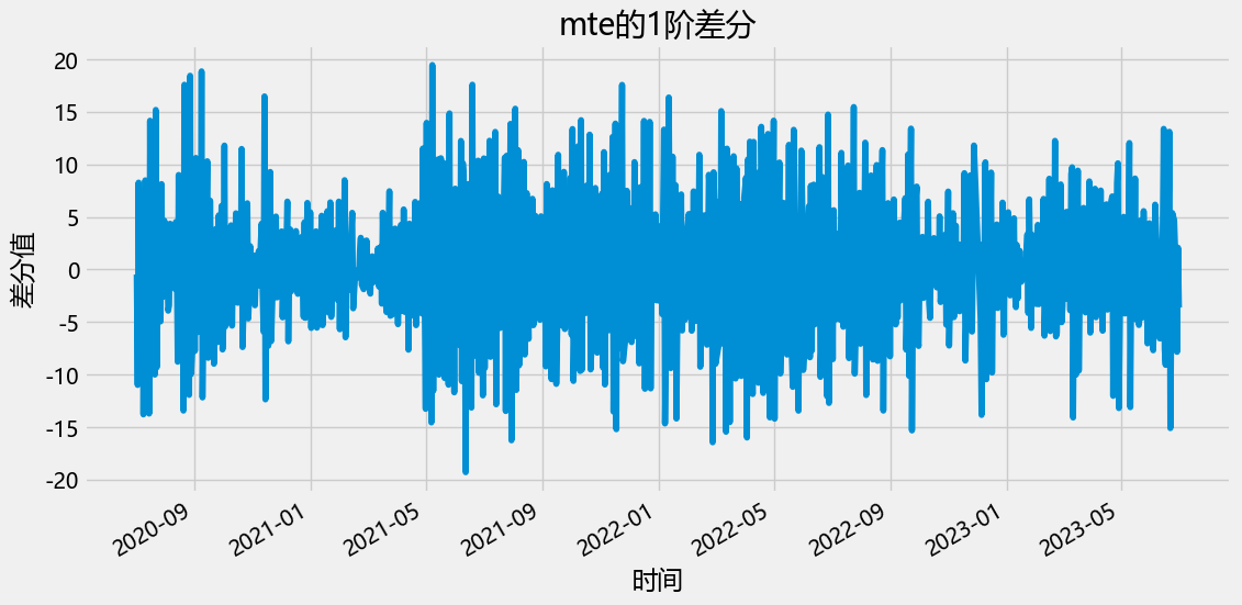
1 2 3 4 5 6 7 8 1 12 , 6 ))'时间' )'差分值' )'mte的{}阶差分' .format (n))
1 2 3 4 5 6 7 8 9 10 11 12 13 from statsmodels.tsa.stattools import adfullerprint (adfuller(mte)) 1 )0 )print (adfuller(diff_mte)) 2 )0 )print (adfuller(diff_mte))
(-3.5123330642834665, 0.0076759468952771045, 22, 951, {'1%': -3.4372448882473177, '5%': -2.86458394997689, '10%': -2.5683907715382888}, 5430.473818612123)
(-11.303446954655314, 1.2904956838904833e-20, 20, 953, {'1%': -3.4372303791313144, '5%': -2.864577551835195, '10%': -2.568387363624452}, 5440.881609824835)
(-10.100507945721994, 1.0625845001080854e-17, 21, 952, {'1%': -3.437237626048241, '5%': -2.8645807475403657, '10%': -2.56838906578808}, 5453.993133667267)
lb_stat
lb_pvalue
1
13.264556
2.704715e-04
2
15.336045
4.675415e-04
3
77.194434
1.226578e-16
4
78.470120
3.673116e-16
5
127.710337
7.284033e-26
6
350.755828
1.062214e-72
7
350.779129
8.392901e-72
8
354.785547
8.616264e-72
9
382.005900
9.428833e-77
10
386.841863
5.931807e-77
11
415.452323
3.198840e-82
12
486.177152
1.934649e-96
13
486.845405
9.088943e-96
14
491.997637
4.602727e-96
15
507.631055
1.373325e-98
16
517.769707
5.873673e-100
17
543.420004
1.313874e-104
18
579.755892
1.628993e-111
19
580.760929
5.765443e-111
20
588.684037
6.953955e-112
1 2 3 4 5 from statsmodels.tsa.arima.model import ARIMA6 ,2 ,4 ))
SARIMAX Results
Dep. Variable: 批发价格(元/千克) No. Observations: 974
Model: ARIMA(6, 2, 4) Log Likelihood -2809.138
Date: Sat, 09 Sep 2023 AIC 5640.277
Time: 18:14:10 BIC 5693.950
Sample: 0 HQIC 5660.704
- 974
Covariance Type: opg
coef std err z P>|z| [0.025 0.975]
ar.L1 -1.8373 0.052 -35.602 0.000 -1.938 -1.736
ar.L2 -1.7422 0.070 -25.023 0.000 -1.879 -1.606
ar.L3 -1.5266 0.078 -19.472 0.000 -1.680 -1.373
ar.L4 -1.3134 0.075 -17.574 0.000 -1.460 -1.167
ar.L5 -1.0602 0.064 -16.448 0.000 -1.187 -0.934
ar.L6 -0.3846 0.038 -10.176 0.000 -0.459 -0.311
ma.L1 -0.0594 0.051 -1.172 0.241 -0.159 0.040
ma.L2 -1.9379 0.047 -40.987 0.000 -2.031 -1.845
ma.L3 0.0592 0.050 1.184 0.237 -0.039 0.157
ma.L4 0.9383 0.047 20.089 0.000 0.847 1.030
sigma2 18.3853 0.845 21.760 0.000 16.729 20.041
Ljung-Box (L1) (Q): 0.04 Jarque-Bera (JB): 70.04
Prob(Q): 0.85 Prob(JB): 0.00
Heteroskedasticity (H): 0.91 Skew: 0.44
Prob(H) (two-sided): 0.40 Kurtosis: 3.98
1 2 3 4 5 6 7 8 9 10 11 12 13 14 15 16 17 18 19 20 21 22 23 24 import pandas as pdimport statsmodels.api as sm'Summary' : [summary],'Parameters' : [params],'Residuals' : [resid],'Fitted Values' : [fitted_values]import osif not os.path.exists('arima result' ):'arima result' )'arima result' + '/' + classname +'model' + '.xlsx' False )print ("ARIMA 结果已成功保存到 Excel 文件:" , filename)
ARIMA 结果已成功保存到 Excel 文件: arima result/食用菌model.xlsx
1 2 from scipy.stats import shapiro
ShapiroResult(statistic=0.9777379631996155, pvalue=4.7044611262148095e-11)
1 2 import statsmodels.api as smprint (sm.stats.durbin_watson(resid.values))
2.002641556155693
1 2 3 4 5 6 7 '2020-07-01' ,'2023-06-30' )12 , 8 ))
[<matplotlib.lines.Line2D at 0x281ab771248>]
1 2 3 4 5 6 7 7 )print (forecast_diff)1 ] + forecast_diff.cumsum()print (forecast)
974 1.130631
975 8.002398
976 0.088760
977 -4.959126
978 -1.411014
979 -0.556519
980 1.472372
Name: predicted_mean, dtype: float64
974 2.262383
975 10.264781
976 10.353540
977 5.394414
978 3.983400
979 3.426881
980 4.899254
Name: predicted_mean, dtype: float64
1 2 3 4 5 6 7 8 9 10 11 12 import osif not os.path.exists('arima result' ):'arima result' )'arima result' + '/' + classname +'result' + '.xlsx' False )print ("ARIMA 结果已成功保存到 Excel 文件:" , filename)
ARIMA 结果已成功保存到 Excel 文件: arima result/食用菌result.xlsx